In condition monitoring and predictive maintenance, vibration analysis is one of the most powerful tools for detecting mechanical faults early. However, technicians and reliability engineers often encounter unexpected challenges, that is two vibration analyzers measuring the same machine under similar conditions can report noticeably different values. These discrepancies can generate confusion, misdiagnosis, or mistrust in the instrumentation if not properly understood. Reliability experts therefore discourage mixing instruments when trending vibration baselines and alarms must be base on a consistent measurement system.
Vibration between devices is normal and often expected. Measurement differences between vibration analyzers commonly arise from hardware/software factors like sampling rate, lines of resolution, and ADC & dynamic range/anti-aliasing implementation. Understanding why readings differ helps organizations standardize their data collection, interpret measurements correctly, and choose the right tools for their maintenance strategy.
Sampling Rate and Anti-Aliasing
Modern vibration analyzers convert the analog signal from an accelerometer into digital data by sampling it. The speed at which samples are taken, the sampling rate, determines the highest vibration frequency that can be measured accurately. If the sampling rate is too low, the analyzer cannot correctly represent fast-changing signals, and distortion appears in the spectrum.
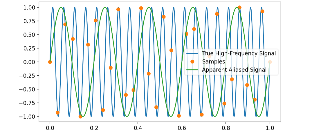
To capture a vibration signal without distortion, the sampling frequency must be a t least twice the highest vibration frequency of interest. Half of the sampling rate is known as the Nyquist frequency. When vibration components exceed this limit, they fold back into the spectrum at lower frequencies. This phenomenon is called aliasing.
Aliasing occurs when a high-frequency vibration appears in the spectrum as a completely different, lower frequency. The analyzer essentially “mistakes” the higher component for something else because it is sampling too slowly. The aliased value always lands somewhere below the Nyquist frequency, which can make the resulting spectrum misleading.
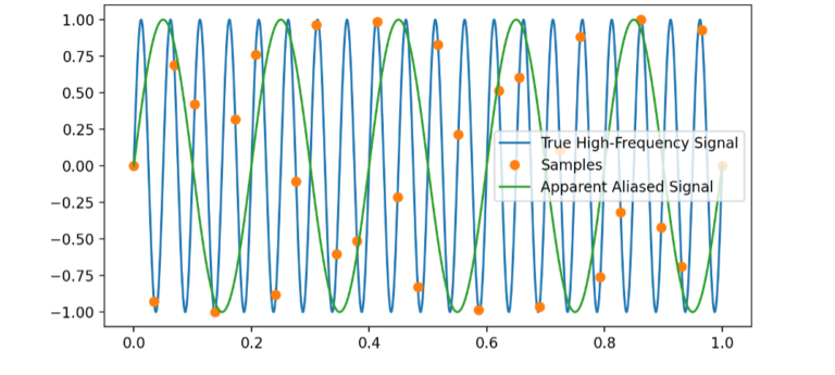
Not all analyzers handle high-frequency content the same way. Differences in sampling rate, anti-alias filtering, and filter steepness can completely change how an allayer responds to frequencies above its Nyquist limit. An analyzer with a strong, modern digital filter sharply suppresses unwanted frequencies, while one with a weak analog filter may allow some high-frequency energy to leak through, creating artificial peaks. This is why two devices measuring the same machine can sometimes produce conflicting results.
Example:
Imagine a machine with a strong vibration at 6,200 Hz.
An analyzer sampling at 25.6 kHz can capture this accurately because its Nyquist frequency is much higher than 6,200 Hz.
Another analyzer sampling at only 12 kH has a Nyquist frequency of 6 kHz, so the 6,200 Hz component exceeds its limit and gets aliased to 5,800 Hz.
A third analyzer sampling at 10 kHz performs even worse: its Nyquist frequency is only 5 kHz, so it reports the signal at about 3,800 Hz far from the true value.
The above example shows how different sampling rates can affect high frequency peaks. Such discrepancies directly affect fault diagnosis, particularly in high frequency bearing analysis. Anti-alias filters are designed to block frequencies beyond the Nyquist limit before the signal is digitized. The quality of this filter determines how high-frequency energy is suppressed. The result is that some analyzers provide clear, reliable high-frequency spectra, while others may distort amplitude, reduce components near the cutoff, or introduce false peaks.
It is important to select the analyzer.
Lines of Resolution
Once a signal is recorded, analyzers use the Fast Fourier Transform (FFT) to convert time-waveform data into a frequency spectrum. The clarity of this spectrum depends on the FFT line resolution, which describes how finely the frequency axis is divided.
FFT resolution depends on both the sampling frequency and the number of samples used. A smaller frequency of bin size results in higher resolution. When resolution is high, vibration peaks appear sharp and accurate. When it is low, peaks become broad or weakened because their energy is spread across multiple bins.
Why Two Analyzers May Show Different Peak Amplitudes
Consider two analyzers measuring up to 5 kHz. One uses 3,200 lines of resolution, while another uses only 800. The second analyzer has bins four times wider, so a vibration peak that does not fall exactly in the center of a bin becomes smeared, causing its measured amplitude to drop significantly.
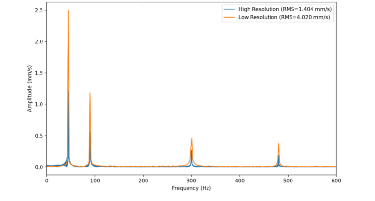
In practice, this can produce errors of 20-30% or more. This happens even when both analyzers are sampling at the same rate. For example, suppose the true peak is at 120.4 Hz with an amplitude of 0.20 g. A high-resolution analyzer might measure nearly the exact same value because the nearest bin is extremely close.
A low resolution analyzer, however, may only land within several hertz of the true value. The resulting energy spreads into multiple bins, causing the peak to appear at 0.14-1.16 g instead. Even though the machine’s behavior has not changed, the analyzer’s resolution make it look different.
When a frequency doesn’t fall perfectly into a bin, some of its energy leaks into the surrounding bins. This is a normal consequence of the FFT process and varies with the chosen window type. Low resolution spectra suffer the most because their bins are wide. Peaks can appear flattened, sidebands may disappear, and broadband noise levels can look artificially high. This greatly affects the ability to diagnose faults such as bearing defects, gear sidebands, or low-speed harmonics.
Other Factors Affecting the Data Variability Between Analyzers
Sensor and Mounting Difference: Analyzers use different transducers; piezoelectric (IEPE) accelerometers and MEMS accelerometers have different bandwidths and noise characteristics resulting in slightly different results for the same equipment. Also, the mounting method significantly affects measurement accuracy, particularly at higher frequencies. Stud-mounted sensors provide the most consistent and accurate data, while magnetic mounts slightly reduce high-frequency transmission. Handheld probes produce the most variability because pressure and angle change easily.
Calibration and Instrument Health: Accelerometers and analyzers naturally drift over time to produce noticeably different vibration readings. This drift can mislead analysts into thinking machine conditions have changed when the instrument is actually out of spec. Also, low battery voltage or aging electronic components can alter the signal path inside the analyzer. These issues may introduce noise or change the device’s gain, affecting measurement accuracy.
Data Processing: Some analyzers average spectra or use overlap/decimation by default; others show single acquisitions. Averaging will reduce random noise and change apparent amplitudes. Vendors choose default windows (Hanning, Hamming, etc.). Different windows trade main-lobe width vs side-lobe levels; with coarse lines, window choice impacts peak amplitude.
Machine and Environmental Factors: A machine is never in a perfectly identical operating state, even minutes apart. Small variation in load, speed, temperature, and nearby activity can influence its vibration signature. Some analyzers respond differently to these transient conditions due to their sensitivity or filtering. Difference in sensor placement, mounting force, and surface conditions further contribute to inconsistent measurements.
Operator-Dependent Differences: Operator technique has a major impact on measurement consistency. Small differences in sensory placement or angle can noticeably affect vibration amplitude, especially at high frequencies. Variations in pressure, cable handling, or choosing slightly different measurement points also introduce variability.
How to Reduce Variability Between Analyzers
There are a couple of steps teams can take to minimize discrepancies and improve data consistency:
Standardize collection procedures: Create a formal procedure defining sensor type, mounting method, measurement points, FFT settings, averaging rules, and units and scaling.
Use the same analyzer for trending: Even if two analyzers are both accurate, they may not trend identically. In machine condition monitoring consistency matters more than absolute precision.
Calibrate regularly: Annual or semiannual calibration of equipment ensures confidence in long-term data.
Train operators: Even small technique difference create big measurement changes, therefore train operators on proper technique.
Conclusion
Differences between vibration analyzers are not only common, but they are completely normal. Variations arise from sampling rate, lines of resolution, and anti-aliasing implementation. Additionally, sensor type, software algorithms, calibration, environmental conditions, and human technique can affect the results. Understanding these actors empowers reliability teams to interpret their data with greater confidence, avoid false assumptions, and build more consistent and trustworthy condition monitoring programs.
Erbessd WiSER and Phantom System
The Erbessd Phantom® Gen 3 sensor provides a sufficiently high sampling rate and adequate spectral resolution to reliably identify common machinery faults, making it well suited for standard condition monitoring programs. With sampling rates up to 25 kHz, frequency ranges reaching 10 kHz, and FFT resolutions up to 12,800 lines, the Phantom® sensor can effectively detect imbalance, misalignment, looseness, and early-stage bearing faults. Its triaxial vibration capability, combined with temperature measurement and wireless installation, long battery life, robust industrial design, cost-effectiveness, enabling scalable deployment across large asset populations. For very high-speed equipment or advanced diagnostic work requiring ultra-high frequency detail and deeper analytical resolutions, the WiSER sensor is recommended due to its superior bandwidth, higher sampling capacity of 48kHz, lines of resolution up to 3,000,000 and enhanced diagnostic performance.
About the Author
Parag Nikam, MS, ISO CAT-1 VA is an IIoT Application Engineer at Erbessd Instruments, where he focuses on delivering condition monitoring solutions designed to meet customer requirements and provides technical support to customers across the globe.
With extensive experience in the reliability engineering field, Parag has worked across diverse manufacturing environments implementing vibration monitoring, predictive/preventive maintenance strategies, and data-driven reliability initiatives. He holds a master’s degree in Mechanical Engineering and has a strong interest in Industry 4.0 and continuous improvement methodologies to enhance asset performance and operational reliability.
ERBESSD INSTRUMENTS® is a global manufacturer of Vibration Analysis Equipment, Dynamic Balancing Machines, and Condition Monitoring solutions, with facilities in Mexico, United States, UK, Colombia and India.